How are the results of Monte Carlo simulations of portfolios affected by the underlying probability distributions of the returns?
The reality we experience is only one manifestation of an infinite number of different paths. This assumption is more likely to be associated with a philosophical debate or the many worlds interpretation of quantum mechanics, but not necessarily with one of the standard methods of the financial industry. We are talking about the Monte Carlo simulation. In this article, we will shed light on this technique and present an online tool that you can use to simulate possible future scenarios for your stock/ETF portfolio yourself.
The procedure of Monte Carlo simulation was already published in 1949 by the scientists Metropolis and Ulam. [1] It is a method of mathematics in which a large number of random experiments are simulated according to a probability distribution. The results are then used to generate possible future scenarios.
To illustrate the process, we can consider the Saturday lottery draw as a Monte Carlo simulation in the physical world. Here, drawing a lottery ball corresponds to the random experiment mentioned above. However, since six balls are drawn in the lottery drawing rather than a single ball, the simulation of a possible scenario or path consists of successively drawing six balls. If we repeat this process several times, the result is a corridor of possible future scenarios and from this we can deduce how probable a particular scenario is.
In the lottery example, drawing “six correct numbers” would be an extreme scenario, because only very few paths lead to this result, while drawing no correct number is most likely, because most of the paths result in this scenario. Thus, one should come to the decision not to play the lottery. Besides these “simulations” in the physical world, Monte Carlo simulations with a large number of scenarios can be simulated with computers. We will use the lottery example again further below to describe the procedure for simulating stock returns. Instead of a lottery number, each ball can be labeled with a monthly return. Then drawing a lottery ball would correspond to randomly determining a monthly return.
What are the preconditions for simulating the development of the stock market with the help of the Monte Carlo simulation? First, we must assume that the stock market’s price development is random. This assumption is widespread among scientists, but it is not uncontroversial. [2],[3] However, if we make this assumption and we know the probability distribution underlying the returns, we can simulate the possible evolution of the stock market. If the number of simulated scenarios is large enough, insightful findings can be obtained.
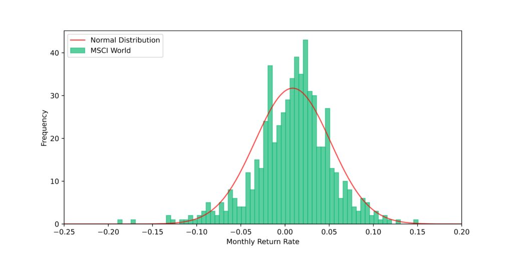
In the last blog entry, we already determined a probability distribution for the returns of the global stock market. We used the MSCI World data of the last 50 years and derived a normal distribution from it, which provides in general a good description of the return distribution. However, stock market crashes with strongly negative returns, such as the Dotcom Bubble or the Great Financial Crisis, are significantly underestimated. The reason is that the distribution of returns is asymmetric or skewed and exhibits a so-called “fat tail” for strongly negative returns. The monthly return distribution of the MSCI World and the normal distribution derived from it with an expected value of 0.87% and a standard deviation of 4.3% are shown in Figure 1.
Since strongly negative returns are significantly underestimated by the normal distribution, we will run on the one hand Monte Carlo simulations relying on the normal distribution and on the other hand by relying on the actual return distribution. Based on the results, we can then assess whether the underrepresentation of months with strongly negative returns by the normal distribution has a decisive impact on the performance or the risk of a portfolio.
The Method of the Monte Carlo Simulation for Portfolios
In the context of the Monte Carlo simulation, each possible path or future scenario consists of a sequence of random events weighted according to a probability distribution. In the simulation of a stock portfolio, the random events correspond to the random determination of a return. We will restrict ourselves to the monthly evolution of the return and consider the evolution of the portfolio for a period of 360 months, respectively 30 years. For our Monte Carlo simulation, this means that we need to randomly generate 360 monthly returns for each path according to one of the two probability distributions described above.
Figuratively, the process for the MSCI World actual return distribution can be thought of as follows. The distribution of actual returns, shown in green in Figure 1, consists of 613 monthly returns. Theoretically, one could get 613 balls and write one of the past returns of the MSCI World on each of them. Using a lottery drum, we could then randomly draw one of these balls. After each draw, the drawn ball is put back and the whole thing is repeated 360 times. This would then be the result of a single Monte Carlo simulation. For the normal distribution, one can proceed in the same way, the balls in the drum would only have to be weighted according to the normal distribution.
In the simulations, we assume that the return is an independent variable, i.e. the return of one month does not depend on the values of the returns of past months, respectively there are no correlations between the returns of different months. This assumption can be doubted if one looks, for example, at a long-lasting so-called bear market, in which prices consistently decline over a long period of time. We will look at how to incorporate such correlations into the model and how they play out in an upcoming blog post.
Since the process with the balls would be somewhat tedious and time consuming, we will use a computerized random number generator that can generate random returns according to the two distributions, but can achieve this far more efficiently. In total, we will run 10,000 Monte Carlo simulations for each of the two distributions, i.e. we will obtain 10,000 possible future scenarios for our portfolio each, based on the past performance of the MSCI World.
Of course, no one can know whether the MSCI World or the stock markets in general will develop similarly in the future as they did in the past. But since we do not have any other data or know any general laws concerning the stock market, the past provides the only possibility to gain knowledge. And with the Monte Carlo simulation we have a powerful tool to derive possible future scenarios from it.
Analysis of the Results of the Monte Carlo Simulations
In this section, we will analyze the results of the Monte Carlo simulations. We will compare the results of the simulations based on a normal distribution with the results obtained from simulations based on the actual return distribution.
Animation of the Monte Carlo Simulation
To illustrate the process of the Monte Carlo simulation, you can watch a video with an exemplary simulation based on the normal distribution. We start with a portfolio value of 100 monetary units. On the left side you can see the normal distribution and a histogram of the simulated or randomly drawn returns, which slowly builds up over time. On the right side you can see the corresponding development of the portfolio value. With increasing time, the compound interest effect can be observed very nicely, since the absolute value of the portfolio now fluctuates much more strongly than at the beginning.
Chart Development
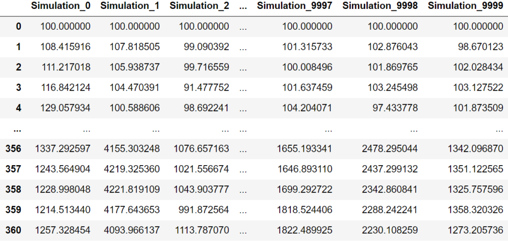
Table 1 shows exemplary results of Monte Carlo simulations with the normal distribution. The whole table has a total of 10,000 columns, one for each possible future scenario and 361 rows, one for each simulated month (the first row contains the initial value of the portfolio). From the last row we can already see that the final value of the portfolio after 30 years can vary a lot.
Of course, we cannot present all values in tabular form here due to the quantity of data points. However, in order to get an overall impression of the results of all simulations, Figure 2 shows the value developments of all 10,000 possible future scenarios. Since portfolio values may have grown considerably after 30 years of compound interest, we have used a logarithmic scale to also observe the development of very poorly performing portfolios with low absolute value. In the animation above, on the other hand, we have used a linear scale. The range of final values covers values from 70 monetary units to almost 50,000 monetary units. It is important to note that these are nominal values, that are not adjusted for inflation.
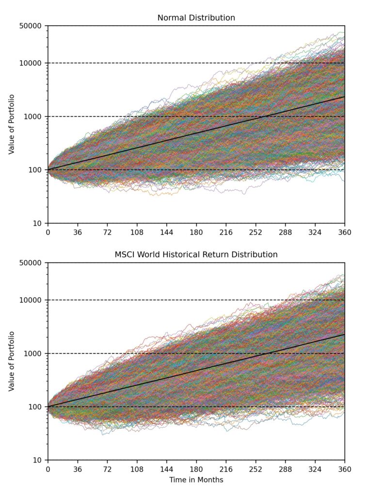
At first glance, the overall picture of all simulations between the normal distribution and the actual return distribution is not really distinguishable, except that for the actual returns, extreme scenarios where the final portfolio value is around 100 monetary units are more common. The black line represents the average value of the portfolios for all simulations at the given time. After 30 years, it is 2325 monetary units for the normal distribution and 2252 monetary units for the actual return distribution. So there is no significant difference. This is to be expected because of the identical expected values of both distributions.
Since Figure 2 is very confusing with the totality of all simulations, we consider below a histogram of all portfolio values in the year 20, i.e. 240 months after the start of the simulation. The histogram is practically a cut along all portfolio values at month 240, and the result can be seen in Figure 3.
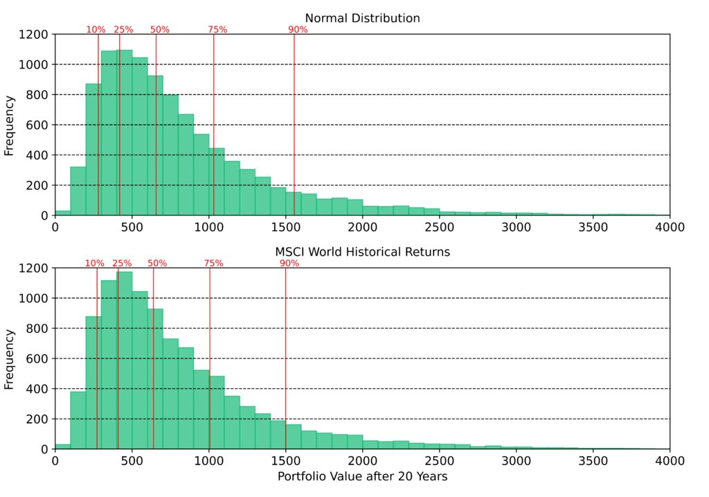
At first glance, the histograms for normal distribution and actual return distribution look identical. Only the quantiles show that the portfolio values after 20 years for the actual return distribution is slightly shifted towards the lower values. Briefly on the meaning of quantiles: For example, the 90% quantile says that 90% of all simulations in the case of the actual return distributions have a portfolio value of up to 1500 monetary units, while this value is about 1550 for the normal distribution. But the difference between normal distribution and actual return distribution is again very small.
Maximum drawdown
Another parameter that plays an important role in the evaluation of stock investments is the so-called maximum drawdown. A drawdown represents the loss between the high and the subsequent low within a certain period. The maximum of these drawdowns is then the maximum drawdown.
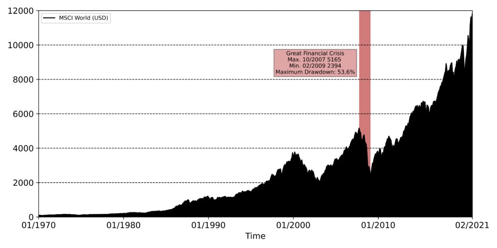
To illustrate the meaning, Figure 4 shows the maximum drawdown for the MSCI World over the last 50 years. It took place at the time of the Great Financial Crisis, peaking in October 2007 and bottoming in February 2009, with a maximum drawdown of a whopping 53.6%.
How does the maximum drawdown behave for our simulated scenarios? Figure 5 shows histograms for the maximum drawdown of all 10,000 Monte Carlo simulations for the normal distribution and the actual return distribution. Looking closely, one can see that for the actual return distribution, small maximum drawdowns up to 37.5% occur significantly less frequently than for the normal distribution. As a result, the average of the maximum drawdowns of all simulations for the actual return distribution is 1.8 percentage points larger.
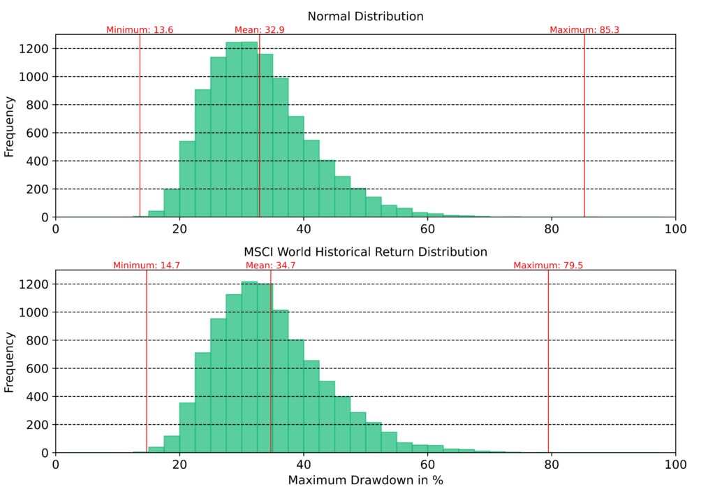
The probability of temporarily higher losses is thus higher in the actual return distribution than in the normal distribution. This is consistent with the underrepresentation of events with strongly negative returns in the normal distribution. The maximum drawdown plays an essential role for investors from a psychological point of view. No investor likes to see a minus of 50% in his portfolio and there is a risk that the investor will actually realize these losses by selling.
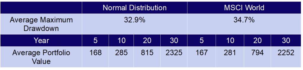
Table 2 summarizes the average portfolio values after 5, 10, 20 and 30 years as well as the maximum drawdown of the Monte Carlo simulations for the normal distribution and the actual return distribution of the MSCI World.
Conclusion
- In this post, we have looked at Monte Carlo simulations for stock portfolios and investigated whether the results differ depending on whether the actual return distribution or a normal distribution is used.
- From Table 2, we can see that the portfolio values and corresponding quantiles at different points in time do not show substantial differences.
- The only variable that shows a significant difference is the maximum drawdown, whose average value for the actual return distribution is 1.8 percentage points larger and high temporary losses are thus more frequent.
- At the outset, we mentioned that in our Monte Carlo simulations we assume that the monthly returns are independent. However, since we have observed prolonged bear and bull markets in the past, the question arises to what extent past returns and future returns are correlated. In an upcoming blog article, we will look at the distribution of the time length of certain stock market phases. We will investigate whether these can be reproduced with an independent distribution of returns or whether we need to add correlations to our simple Monte Carlo simulation. For example, does a negative return follow a negative return with 50% probability?
- One book I can strongly recommend on the subject of Monte Carlo simulations for portfolios and the role of randomness in life is the book “Fooled by Randomness” by author Nassim Nicholas Taleb (see book recommendations for more information).
- There are tools on the Internet that allow you to run Monte Carlo simulations for stock portfolios online. See financial tools for more information.
Have you ever used Monte Carlo simulations to simulate possible future scenarios for your stock portfolio, ETF savings plans or withdrawal plans? Let me know in the comments.
Sources
[1]: Metropolis, N. C./Ulam, S. (1949): The Monte Carlo Method, Journal of the American Statistical Association, Vol. 44, No. 247, (Sep. 1949), S. 335-341.
[2]: Cootner, Paul H. (1964). The Random Character of Stock Market Prices
[3]: Lo, Andrew (1999). A Non-Random Walk Down Wall Street